
Yingjun Mou


Simulation of Rodent Plague in Manhattan with Population Dynamics Models
Group Project for A-4834 Data Mining the City 12/2018
 plague simulation of Manhattan with different conditions
Introduction
The purpose of this project is to simulate the spread of potential rodent plague in Manhattan. With 311 data on reported rat sightings, we are able to recognize the locations where the sources of infection might be. The population dynamics simulation will be the main tool to illustrate the spreading trend of the epidemics and help us to know how to apply direct and immediate response toward the emergent accident. This report aims to address the following research questions:
- Who will ultimately get infected according to the existing condition and the assumption?
- What is the minimum number of infected people that will result in the whole neighborhood getting infected?
- How will the cure rate and human fluidity influence the spread of the plague?
- How will different patterns of movement (day or night) or different groups of people (senior citizens, children) influence the spread of plague?
Regarding the rodent plague as a case study, this prototype has its potential to serve as a template for other epidemics.
Background
From the 1900 San Francisco bubonic plague epidemic to the 2012 Yosemite National Park hantavirus outbreak, rats can spread diseases and compromise public health (Brown and Laco 2015). In United States, most plague happen in the rural west, and the rodent associated plague in Los Angeles during 1924–1925 is recorded to be the last outbreak in urban areas.
New York City’s rodent problem is infamous. A research shows that there are around 2 million rats in total in New York City, which is approximately 24% of the number of humans (Auerbach 2014). Rats inhabiting in New York all belong to the same species, Rattus norvegicus or Norwegian rat. These rats have a high rate of reproduction and are hard to kill since they can scamper around underground tunnels and dense buildings. Furthermore, rodent problem is also one of the top concerns for citizens. From the beginning of 2017 to November 2018, around 876,000 complaints are recorded through the 311 system in Manhattan. Rodent related complaints, including rat or mice sightings and signs of rodents, is among the Top 20 concerns and comprises around 1.6% of total records.
Though plague is not common in cities, considering the large population of rats in New York, it is of importance to understand the distribution of the rodent community and to simulate the spread in order to better response to potential outbreak.
Literature Review
In order to show the mobility of human beings and the change of their infection status, this research is based on an agent-based population dynamic modelling using the structure of cellular automata. A cellular automaton consists a grid of cells, each of which is in a finite number of states. And fundamentally the automaton can be defined as a triplet: <'I, S, W>, where I is the set of inputs, S is a set of states and W is the next-state function, depending on the input and state pairs (Hogeweg 1988).
Cellular automata was first designed in the 1940s and the most well-known work is the Conway’s Game of Life in the 1970s, which also led the interest in this subject to extend into the academic world and many other research fields. Previous studies have shown that cellular automata has become a powerful tool to simulate complicated spatial-temporal problems, such as ecological process (Hogeweg 1988) and land use change (White and Engelen 1993) since it is structured on simple rules but can produce diverse behaviors and patterns. CA is also used as a bottom-up approach to model population dynamics. Under such a framework, the model city is populated by agents that can move, change their state, and imitate their neighbors (Benenson 1998) and this provides the theoretical basis of this rodent plague research.
The selection of a suitable modeling formalism is related with certain research area. There are two reasons to choose CA in this project other than classical models. First, CA could best preserve the locality of both variables and interactions, as well as provide a way to view the interaction globally (Green 1990). Different from classical models which center on the original variables and the algebraic form of interactions (linear or nonlinear analysis), CA creates an environment for variables and interactions with all the variables in the original location (Hogeweg 1988). The number of variables is big, while for each of the variables, the number of states of is generally small (Hogeweg 1988). Second, CA could encompass multilevel modelling in the study. Most classical one-level models are formed by observed variables and illustrate the interactions among the observed variables. On the contrary, CA formulates a more dynamic scenario — variety of behavior were depicted in the model and the variables tend to be “self-organized” (Green 1990). New populations are distributed in the locality follows an algorithm of the original variables (Ruiz-Moreno et al. 2002).
Simulation Model Design
(A)Data Structure
There are two interfaces: the individual in a micro scale (represented using class “Person”) and the City in a macro scale (represented using class “Population”). While the “Person” has a “state” variable to indicate his/her health condition, the “Population” has a series of functions to achievement the dynamic interactions between different “Person” objects.
Class “Person”:
- state— healthy if state=0, being infected if state=1, infected if state ≥2
- checkState ()— observer of current state
- changeState()— modifier of current state
Class “Population”:
- maxX, maxY — dimension of the 2D matrix representation of population
- countAdj —given a specific person, count the number of infected people adjacent to him/her
- eval — evaluate the most “influential” infected persons who will directly result in the new infected population the next day
- infect — increase the number of infected population based on our rules of infection
- cured —randomly make infected person healthy based on the cure rate
- move — randomly make people move around to accelerate the infection process
(B)Rules of Infection
- If there are >= 2 out of 4 nearby people infected, then the individuals will be infected the next day (each people is represented as a square pixel)
- After 50 days (one day each frame), an infected person will die
- There is a preset probability of being cured, and a preset probability of moving around(and to spread the disease).
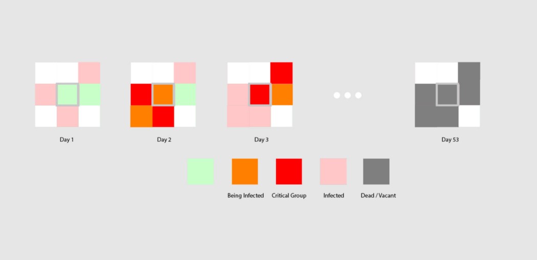 illustration of the infection rules
Data Retrieval & Python Implementation
(A)Data Preparation:
We use R studio and GIS to clean and aggregate the data. 311 rodent complaint dataset on the New York open data is made by Department of Health and Mental Hygiene (DOHMH) and is updated daily since 12/16/2015. To simplify the analyzing process, we extract the complaint data from 2017 to 2018 and spatial join them into census blocks. And several areas are recognized to have more rodent inspection, such as Southern Bronx, Upper West Side, East Village, and Lower East Side.
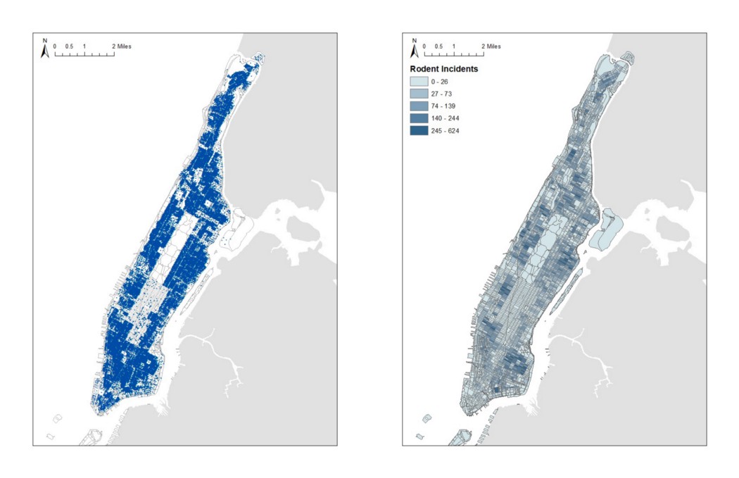 rodent plague incident distribution maps
(B)Simulation:
Manhattan has been divided into 27x72 2D grids. CSV made in previous step is imported in processing and read line-by-line, providing each grid with attribute of its own population density and plague outbreak probability. In each grid, 25 pixels are used to represent the population in each block referring to the ACS data. And locations with higher population density and rodent records have been imported in the processing canvas and acted as the source of infection. Disease cure rate and population fluidity are regarded as the key factors of terminating the spread of plague.
Disease cure rate in this report is presented as percentage format. The 2.5% disease cure rate indicates that in 100 people randomly 2.5 people can be cured in an iteration. Population fluidity is also presented as percentage format. The 50% population fluidity demonstrates that in 100 people, 50 people would randomly move in an iteration.
Different disease cure rates and population fluidity are set in the research process to test the best solution toward quenching the spread of plague. We define 2.5% cure rate as a low level cure rate, 25% cure rate as a high level cure rate; and 10% population fluidity as a low population fluidity, 50% population fluidity as a high population fluidity.
Data and Assumptions
The model is based on the following datasets and assumptions.
(A). Demographic data describes characters of the agent. Population density, median household income and percentage of the old and young in each census block throughout Manhattan are introduced into the model. We assume that:
- Areas with higher population density tends to be the sources of rodent outbreak
- When we calculate the “Critical Group” given the infection condition of a specific day, we assume that at the time of calculation, the population at each neighborhoods are quarantined and thus don’t move at all.
(C). History record of rodent presence. We assume that places where there were more rodent complaints tend to be the sources of plague outbreak.
Expected Output
(A). Visualization of the spread of disease under different mobility levels and cure rates. The hypothesis is that higher mobility would lead to faster plague spread and higher cure rate would curb the process. The interaction of these two factors would also be shown in the simulation model.
(B). Highlight of the “Critical Group” for helping the better vaccine-targeting. “Critical Group” denotes those persons which should be prioritized for being vaccinated in order to minimize the following infected population. For instance, if there are limited medical resources (imagine a new type of panacea which can cure infected people instantly), in order to stop the spreading of disease and minimize the number of infected people, in which neighborhood should the government use the panacea?
Test Samples
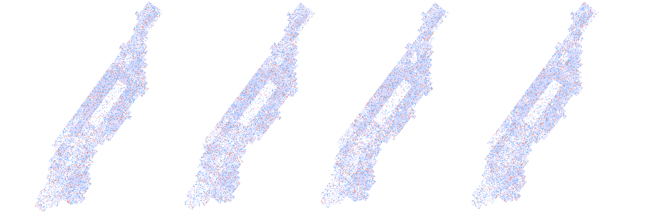
In order to analyze the correlations between cure rate, population fluidity, and the overall infection, we set cure rate to be 2.5%, 10%, 25%, and population fluidity to be 10%, 50%, to establish 5 different test cases.
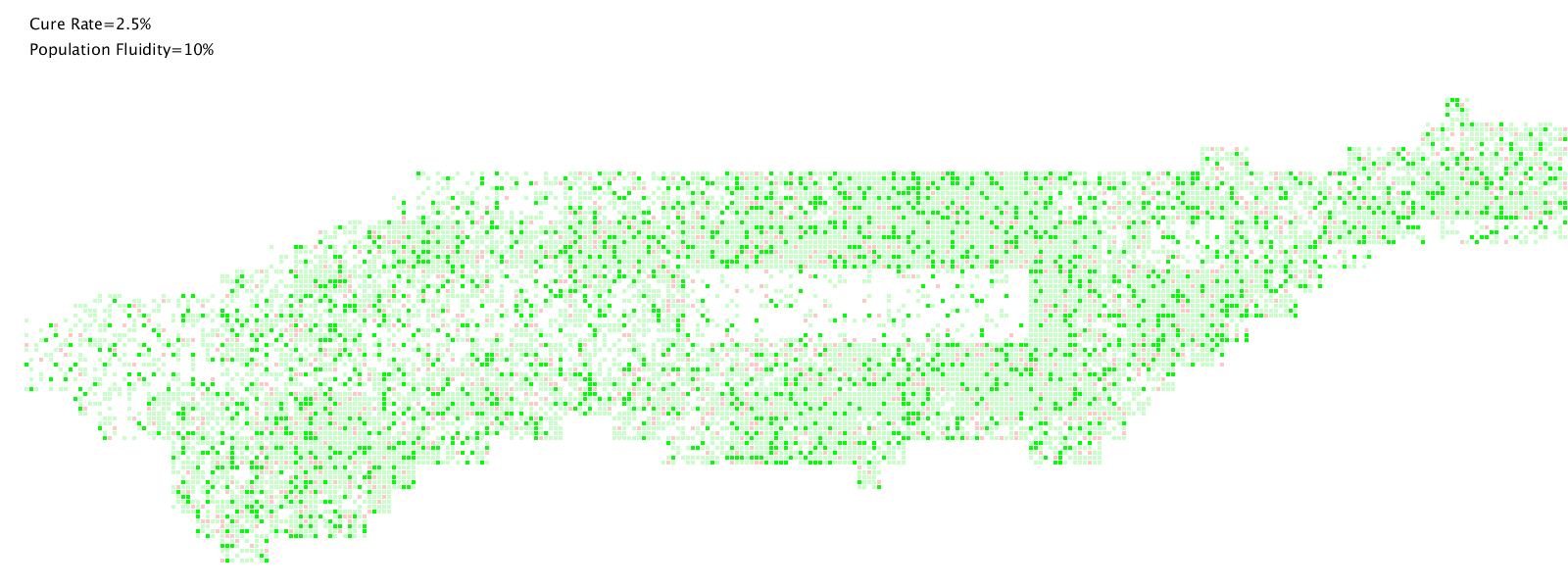 Scenarios A: cure rate=2.5%, population fluidity=10%. Infection spreads in a fair speed and eventually forms clustering of impacted areas.
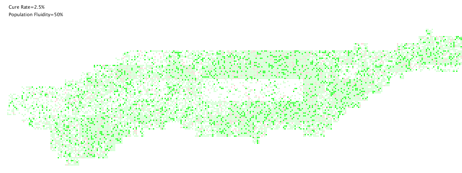 Scenarios B: cure rate=2.5%, population fluidity=50%. Infection spreads quickly and eventually swallows the entire city.
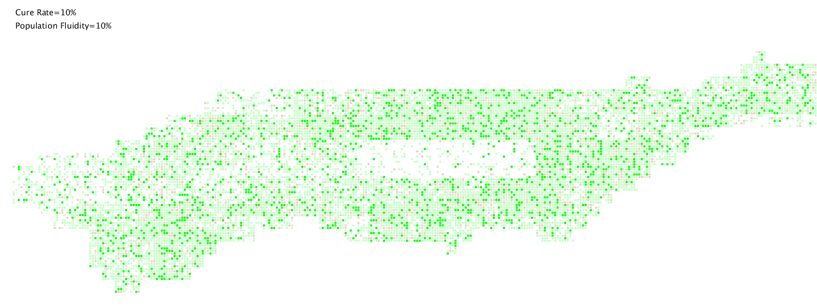 Scenarios C: cure rate=10%, population fluidity=10%. Infection was contained, but not quenched.
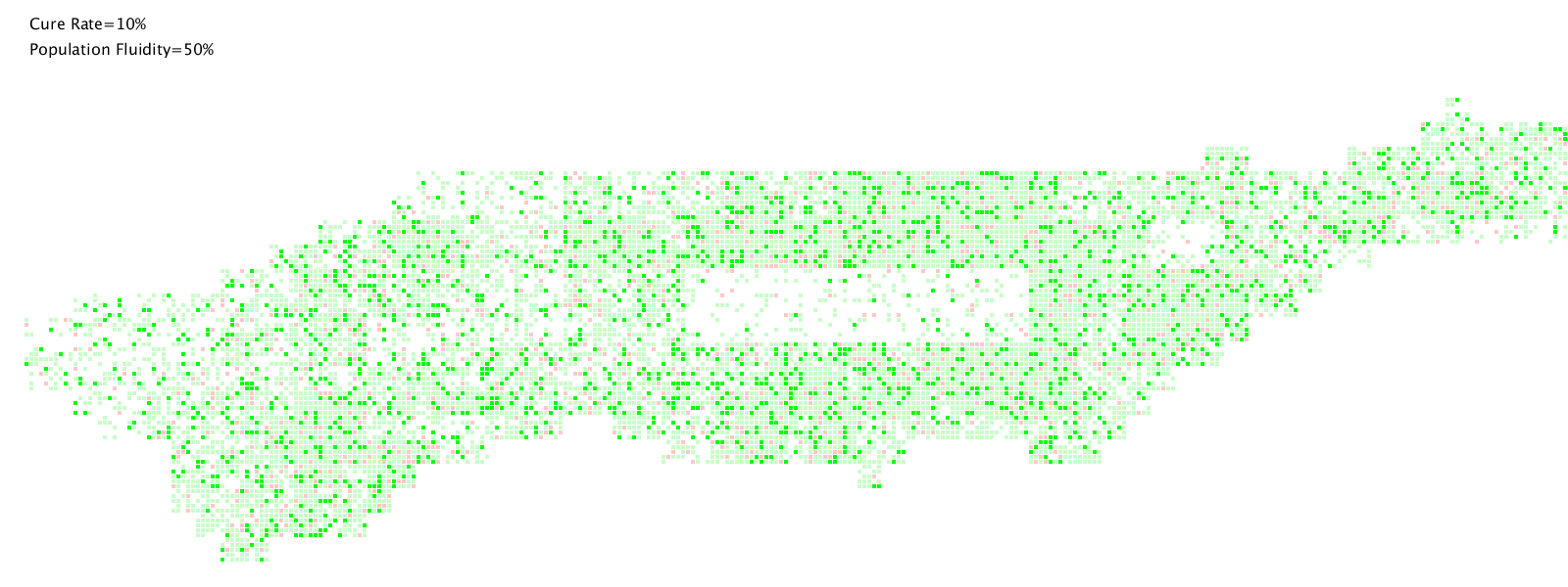 Scenarios D: cure rate=10%, population fluidity=50%. Infection spreads slowly and forms clustering of impacted areas.
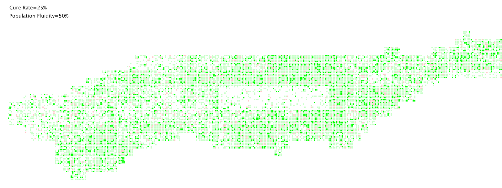 Scenarios E: cure rate=25%, population fluidity=50%. Infection was quickly quenched by the high cure rate.
Conclusion
(A) Based on the history record of rodent plague outbreak, and the population distribution in Manhattan, there are several areas which has a higher probability of suffering from rodent plague, such as Southern Bronx, Morningside Heights, Midtown West, and Lower East Side.
(B) In terms of quenching the spread of plague, the Higher Cure Rate works better than the Lower Population Fluidity. Population Fluidity is more about how fast the plague will spread.
(C) The “Critical Groups” (highlighted using crimson red) are either on the periphery of the infected clusters, or inside the clusters and near those uninfected “porous”. If the medical resources is limited, the government should cure and vaccinated them first in order to minimize the number of following infection.
(D) There are 4 areas which indicate how the population density, geographical condition, and the environmental condition can somehow decided a neighborhood’s fate during an epidemics. For example:
- Wall Street (upper left picture) can easily survive from the epidemics, given that almost 3 sides of it are river and thus isolated from the rest of the city. And it has a fairly low density of population compared with midtown. Thus, it’s very hard for the plague broke out in the north to infiltrate into this area.
- Lower East Side (upper right picture) is one of the areas with the most severe casualties under the circumstance of epidemics. And it’s mainly because there are multiple streets with high volume of incidents in the past, and they are adjacent to each other, which favor for the clustering effect of infected population.
- Upper West Side (lower left picture) can also be a haven from epidemics. Because it has a better environmental condition (fewer incidents of plague outbreaks in the past). And what’s more importantly, it’s also semi-isolated by the river in the north and the central parks in the south, which serve as buffer zones for the infection.
- Morningside Heights (lower right picture), on the other hand, will be easily infected by its surrounding neighborhoods such as East Harlem and Southern Bronx because of the population density makes a continuous pathway for disease to come in.
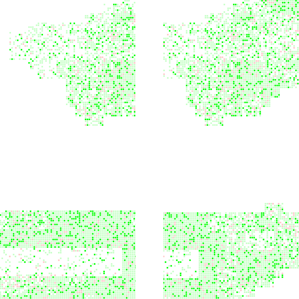 (1) upper left: Wall Street - (2) upper right: Lower East Side — (3) lower left: Upper West Side - (4) lower right: Morningside Heights
Limitation and Extension
We need to admit that this mathematics model for rodent plague simulation has some limitations to some extent.
For example, the simulation is based on a probabilistic model, instead of a deterministic model. All the predictions are largely reliant on the input data, and inevitably has inaccuracy.
And for the simplification of model and computation, the movement of population has been a abstraction of randomly moving along on of the four directions (upward, downward, leftward, rightward), and more complicated movement patterns have been ignored.
We look forward to revisit and improve our simulation model in the future, by studying the patterns population during different times and by enlarging our dataset.